
Matlab analysis of the mass-spring-damper system (time responses based on the analytical solutions)
(1) msd class
To handle multiple configurations of mass-spring-damper systems, it is convenient to define a mass-spring-damper class ‘msd‘ to store properties of the system. In application, the user creates multiple msd instances, each of which corresponds with one configuration of interest.
The code below is the definition of the msd class. The class consists of the three parameters of a mass-spring-damper, namely, the mass \(m\), damper coefficient \(c\) and spring coefficient \(k\). The code also contains methods to calculate other dependent properties of the system, such as the undamped natural frequency \(\omega_{n}\), damping ratio \(\zeta\), transfer function, the root of the characteristic equation \(s\) and the time responses \(x(t)\) due to the step and impulse input forces \(f(t)\).
In the functions ‘Step’ and ‘Impulse’ in the below msd class definition, the time responses are calculated based on the analytical solutions of the differential equation of the system, listed in the left column on the tables in Summary of the analytical solutions
1 2 3 4 5 6 7 8 9 10 11 12 13 14 15 16 17 18 19 20 21 22 23 24 25 26 27 28 29 30 31 32 33 34 35 36 37 38 39 40 41 42 43 44 45 46 47 48 49 50 51 52 53 54 55 56 57 58 59 60 61 62 63 64 65 66 67 68 69 70 71 72 73 74 75 76 77 78 79 80 81 82 83 84 | classdef msd
% Mass Spring Damper Data Set Class
properties
m % Mass [kg]
c % Damper coefficient [N/(m/s)]
k % Spring coefficient [N/m]
end
properties (Dependent)
wn % Undamped natural frequency [rad/s]
wd % Damped natural frequency [rad/s]
zeta % Damping ratio
s % Roots of the characteristic equation
TF % Transfer function
end
methods
% constructor
function obj = msd(m, c ,k)
if nargin > 0
obj.m = m;
obj.c = c;
obj.k = k;
end
end
% dependent properties calculated on request
function wn = get.wn(obj)
wn = sqrt(obj.k/obj.m); % undamped natural frequency [rad/s]
end
function zeta = get.zeta(obj)
zeta = obj.c/(2*obj.m*obj.wn); % damping ratio
end
function wd = get.wd(obj)
wd = obj.wn*sqrt(1-obj.zeta^2); % damped natural frequency [rad/s]
end
function s = get.s(obj)
s = complex( [-obj.zeta*obj.wn + obj.wn*sqrt(obj.zeta^2-1)
-obj.zeta*obj.wn - obj.wn*sqrt(obj.zeta^2-1)] );
% root of the characteristic eq
end
function TransferFunction = get.TF(obj)
TransferFunction = tf(1, [obj.m, obj.c, obj.k]); % transfer function
end
% functions that outputs time responses
function [step_t, step_x] = Step(obj, t, step_value)
% step_value - the magnitude of the input force [N]
% for unit step input set it to 1
% t - time vector at which the step response is calculated
if obj.zeta < 1 % underdamped
theta = atan(sqrt(1-obj.zeta^2)/obj.zeta);
x = step_value/obj.k * (1 - exp(-obj.zeta*obj.wn.*t) .* sin(obj.wd.*t + theta) ./sqrt(1-obj.zeta^2));
elseif obj.zeta == 1 % critically damped
x = step_value/obj.k * (1- (1+obj.wn.*t).*exp(-obj.wn.*t));
else
alpha1 = obj.wn * (obj.zeta + sqrt(obj.zeta^2-1));
alpha2 = obj.wn * (obj.zeta - sqrt(obj.zeta^2-1));
x = (step_value/obj.wn^2) * ...
(1 - (alpha1.*exp(-alpha2.*t) - alpha2.*exp(-alpha1.*t) )./(alpha1-alpha2) );
end
step_t = t;
step_x = x;
end
function [impulse_t, impulse_x] = Impulse(obj, t, scale_value)
% scale_value - the multiplier of the scaled impulse
% for unit impulse set it to 1
if obj.zeta < 1 % underdamped
x = scale_value/ (obj.m * obj.wd) * exp(-obj.zeta.*obj.wn.*t) .* sin(obj.wd.*t);
elseif obj.zeta == 1 % critically damped
x = scale_value/obj.m .*t.*exp(-obj.wn.*t);
else
alpha1 = obj.wn * (obj.zeta + sqrt(obj.zeta^2-1));
alpha2 = obj.wn * (obj.zeta - sqrt(obj.zeta^2-1));
x = (scale_value/(alpha1-alpha2)) * ...
( exp(-alpha2.*t) - exp(-alpha1.*t) );
end
impulse_t = t;
impulse_x = x;
end
end
end |
(2) Example script file (for \(\zeta\) sweep with the step response of \(f(t) = 9 \) N)
The below Matlab script stands as an example of the method to plot the time responses and the root locus using the msd class defined above.
In the first section of the code, several configurations of mass-spring-dampers with changing damper coefficients \(c\) are set, then the time vector against which the time response is calculated are given, along with the magnitude of the input force after the step event \(f(t)\).
In the second section, ‘msd’ instances are created for each of the different configurations of the mass-spring-dampers and the step responses are calculated. The last section of the code allows the visual comparison of the mass-spring-damper systems. Figure (1) is the Root Locus and Figure (2) is the time response based on the functions in the msd class definition. Figure(3) outputs the same time response as Figure (2). The differences are Figure (3) utilises the transfer function of each msd instance in conjunction with the built-in function ‘step’ in the Matlab Control System Toolbox to confirm the result.
1 2 3 4 5 6 7 8 9 10 11 12 13 14 15 16 17 18 19 20 21 22 23 24 25 26 27 28 29 30 31 32 33 34 35 36 37 38 39 40 41 42 43 44 45 46 47 48 49 50 51 52 53 54 55 56 57 58 59 60 61 62 63 64 65 | clear all %% inputs % specification of the mass spring dampers. m[kg], c[Ns/m], k[N/m] mcks = [1 0 9 1 1.2 9 1 3.6 9 1 4.8 9 1 6.0 9 1 7.2 9]; t = [0:0.05:5].'; % time vector for plot of time response step_value = 9; % the magnitude of the input force [N] after step event %% create msd instances and calc time responses num_msds = size(mcks,1); % the number of systems %initialise data store arrays msds(num_msds,1) = msd; % initialise the object array to store instances step_ts = cell([num_msds, 1]); step_xs = cell([num_msds, 1]); for i = 1:num_msds msds(i) = msd(mcks(i,1), mcks(i,2), mcks(i,3)); %create instances of mass-spring-damper systems using 'msd' class [step_ts{i}, step_xs{i}] = Step(msds(i),t, step_value); %calculate the response to step input f = step_value [N] end clear i legend_zetas = strings(num_msds,1); % prepare string array for plot legend zeta_values = [msds.zeta]; for i = 1:num_msds legend_zetas(i) = sprintf('zeta = %.2f', zeta_values(i)); end clear zeta_values %% plots figure(1), clf, hold on plot([msds.s], 'x', 'MarkerSize', 8) legend(legend_zetas, 'Location', 'SouthEast') FormatPlot() xlim([-5 5]), ylim([-5 5]) axis equal title('The roots s of the characteristic equation') xlabel('Real'), ylabel('Imaginary') figure(2), clf %step response using the msd class hold on for i = 1:num_msds plot(step_ts{i}, step_xs{i}) end clear i legend(legend_zetas, 'Location', 'SouthEast') grid on title('Step response') xlabel('Time t [s]'), ylabel('Displacement x [m]') FormatPlot() figure(3), clf, hold on % plot step response using Control System Toolbox opt = stepDataOptions('StepAmplitude',step_value); % alter the step amplitude for i = 1:num_msds step(msds(i).TF, t, opt) % plot time response using built-in function end legend(legend_zetas, 'Location', 'SouthEast') FormatPlot() |
The script uses a small auxiliary function FormatPlot() below, stored in the same directory, to adjust the line width and font size used in the figure windows.
1 2 3 4 5 | function[]= FormatPlot() set(findobj(gcf,'type','line'),'LineWidth', 2); set(findobj(gcf,'type','axes'),'FontSize',16, 'LineWidth', 0.5); grid on end |
Resulting plots from the example script
In the above example script, six mass-spring-dampers with varying damper coefficient were configured, while the mass and spring coefficient were fixed at \(m=1\) kg and \(k=9\) N/m. The damper coefficients range from \(c=0\) to \(c=7.2\) Ns/m, corresponding with no damping \(\zeta = 0 \) to overdamping \(\zeta = 1.2\).
The six mass-spring-dampers share the same natural frequency of \[ \omega_{n} = \sqrt{\dfrac{k}{m}} = \sqrt{\dfrac{9}{1}} = 3 \; \text{rad/s} \]
(1) Root Locus
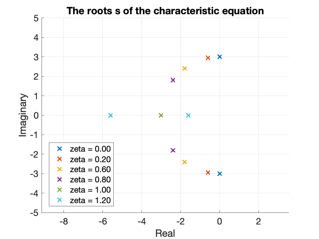
The figure is the root locus formed by the six mass-spring-dampers. The two conjugate roots \(s\) of the characteristic equation \(ms^2+cs+k =0\) lie on the imaginary axis in case of no damping \(\zeta = 0\). With an increase in damping, the conjugate roots shift towards the middle of the figure, while keeping the constant distance \(\omega_n = 3 \) to the origin.
At critical damping \(\zeta = 1\), the two roots meet on the real axis. With further increase in damping the system become overdamped \(\zeta > 1\). One root moves to the left on the imaginary axis, while the other root moves to the right on the same axis.
(2) Time response with step input \(f(t)= 9, t>0\)
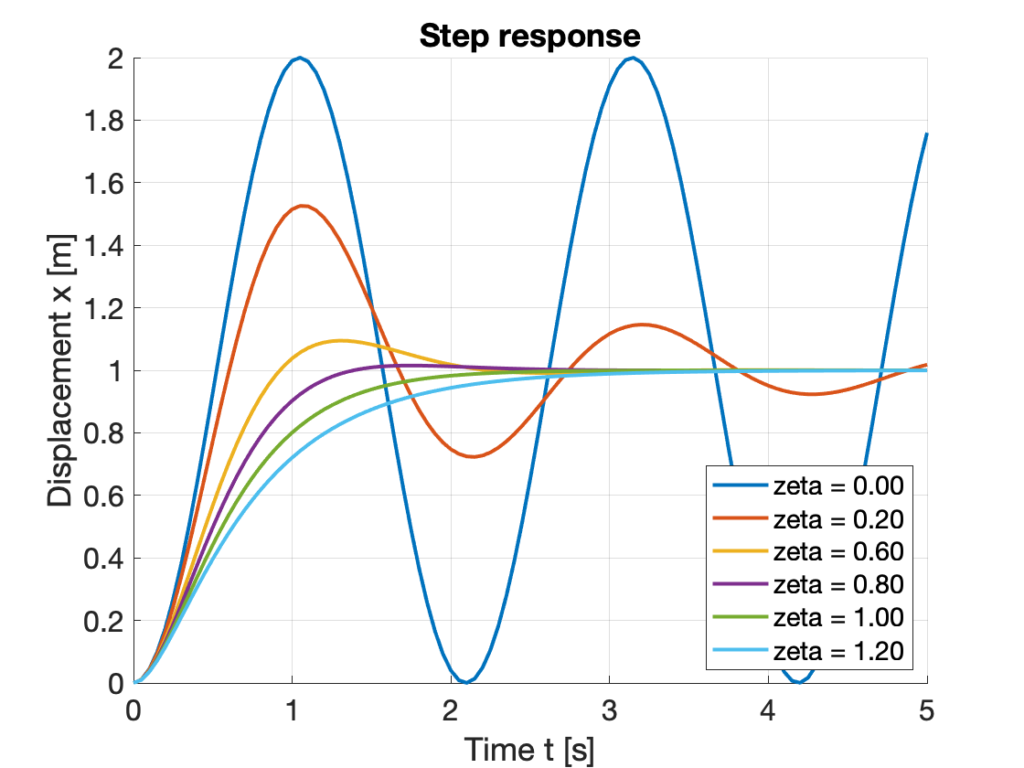
The figure is the time responses of the six mass-spring-dampers. Since the spring coefficient is \(k = 9 \;\text{Nm}\) for all the configurations, the step force input of the amplitude \(f = 9\; \text{N}\) results in a unit steady-state response of \(x =\dfrac{f}{k} = 1 \; \text{m}\).
For no damping case \(\zeta = 0\), the oscillation does not reduce in its amplitude. With an increase in damping, the peak value reduces. At critical damping \(\zeta = 1\), there is no oscillation. With overdamping \(\zeta = 1.2\), there is still no oscillation, however, it takes a longer time to settle to the steady-state than the critical damping. It is notable that at \(\zeta = 0.8\), the system largely reaches the steady-state value quicker than the critical damping except for some minor overshoot.
(3) Time response with unit impulse input \(f(t)= \delta, t=0\)
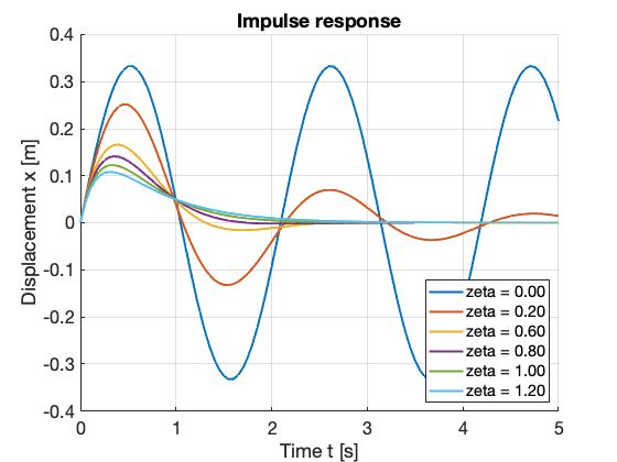
The figure is the time responses of the same six mass-spring-dampers subject to the unit impulse input. Similar to the step input response, the oscillation does not reduce for no damping \(\zeta = 0\) case. The peak value reduces with an increase in damping. At \(\zeta = 0.8\), the steady-state is reached quicker than the critical damping \(\zeta =1\), however, has the higher first peak.